Age-sex pyramids

Introduction

Age-sex pyramids are fundamental tools in epidemiological analysis, providing a visual representation of the demographic distribution of cases. They help identify vulnerable populations, understand transmission patterns, and guide public health interventions. The age_sex_pyramid() function supports both line-list data (individual cases) and pre-aggregated counts so that analysts can tailor output to their workflows.

Prerequisites

library(epiviz)
library(dplyr)
library(lubridate)

Example 1: Static pyramid from line-list data

Static pyramids are ideal for publications and reports where a clear, printable summary of the population structure is required. In this example we subset epiviz::lab_data to Staphylococcus aureus detections recorded during 2023 and let age_sex_pyramid() calculate the age bands automatically from the line-list data.

Prepare the line-list data

line_list_pyramid_data <- epiviz::lab_data %>%
  filter(
    organism_species_name == "STAPHYLOCOCCUS AUREUS",
    specimen_date >= as.Date("2023-01-01"),
    specimen_date <= as.Date("2023-12-31"),
    !is.na(date_of_birth),
    !is.na(sex)
  ) %>%
  mutate(
    sex_clean = case_when(
      toupper(sex) %in% c("M", "MALE") ~ "Male",
      toupper(sex) %in% c("F", "FEMALE") ~ "Female",
      TRUE ~ NA_character_
    )
  ) %>%
  filter(!is.na(sex_clean))

Plot the static pyramid

age_sex_pyramid(
  dynamic = FALSE,
  params = list(
    df = line_list_pyramid_data,
    var_map = list(
      dob_var = "date_of_birth",
      sex_var = "sex_clean"
    ),
    grouped = FALSE,
    mf_colours = c("#440154", "#2196F3"),
    x_breaks = 6,
    x_axis_title = "Number of detections",
    y_axis_title = "Age group (years)",
    chart_title = "Static age-sex pyramid",
    age_calc_refdate = as.Date("2023-12-31")
  )
)

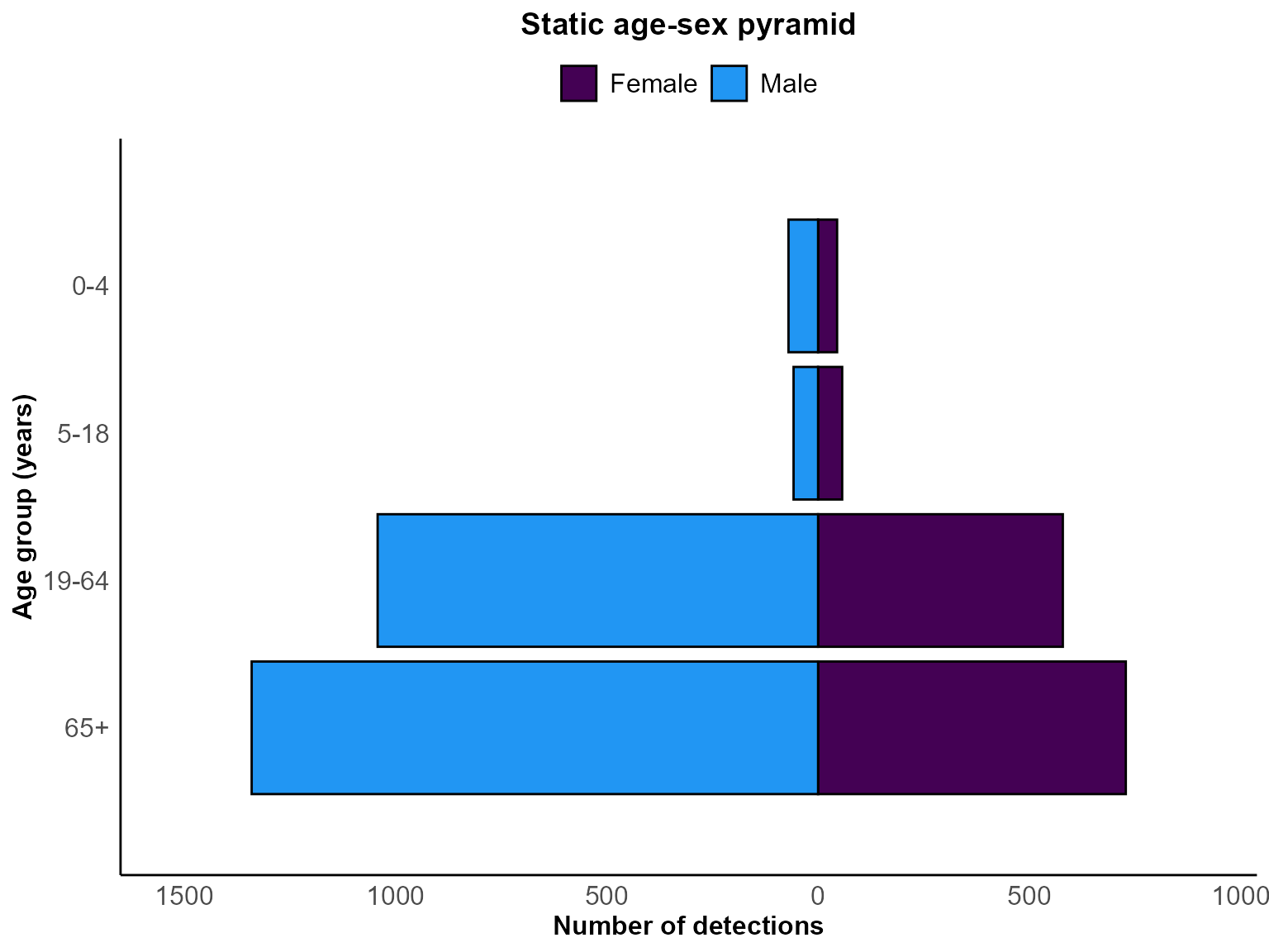
Age-sex pyramid for Staphylococcus aureus detections between January and December 2023.

Interpretation: The plot highlights the age groups contributing most to laboratory detections, with mirrored bars showing the relative burden among males and females.

Example 2: Interactive grouped pyramid with confidence intervals

Interactive pyramids are useful for exploratory dashboards where end users can interrogate the data directly. By aggregating the same records into age bands and providing the associated Poisson confidence intervals, the plot reveals both the central estimates and their uncertainty.

Aggregate counts and calculate confidence intervals

grouped_pyramid_data <- line_list_pyramid_data %>%
  mutate(
    age_years = floor(time_length(interval(date_of_birth, as.Date("2023-12-31")), "years")),
    age_band = cut(
      age_years,
      breaks = c(0, 5, 15, 25, 35, 45, 55, 65, 75, 85, Inf),
      right = FALSE,
      labels = c("0-4", "5-14", "15-24", "25-34", "35-44",
                 "45-54", "55-64", "65-74", "75-84", "85+")
    )
  ) %>%
  filter(!is.na(age_band)) %>%
  count(age_band, sex_clean, name = "val") %>%
  rename(sex_mf = sex_clean) %>%
  mutate(
    lower_ci = if_else(val == 0, 0, qchisq(0.025, 2 * val) / 2),
    upper_ci = qchisq(0.975, 2 * (val + 1)) / 2
  )

Plot the interactive grouped pyramid

age_sex_pyramid(
  dynamic = TRUE,
  params = list(
    df = grouped_pyramid_data,
    var_map = list(
      age_group_var = "age_band",
      sex_var = "sex_mf",
      value_var = "val",
      ci_lower = "lower_ci",
      ci_upper = "upper_ci"
    ),
    grouped = TRUE,
    ci = "errorbar",
    mf_colours = c("pink", "blue"),
    x_breaks = 5,
    chart_title = "Interactive grouped pyramid with CI",
    x_axis_title = "Number of detections",
    y_axis_title = "Age group (years)",
    legend_title = "Sex"
  )
)

Interactive age-sex pyramid with 95% confidence intervals for Staphylococcus aureus detections in 2023.

Interpretation: The interactive plot provides hover labels for precise counts and asymmetric confidence intervals, enabling rapid assessment of uncertainty for each age-sex combination.

Tips for age-sex pyramids

1. Data preparation: For line-list data (grouped = FALSE), ensure your date-of-birth and sex variables are present and clean; the function can derive age groups from dates directly.
2. Variable mapping: Use var_map to align your column names with the expected inputs. Grouped data requires age_group_var, sex_var, value_var, ci_lower, and ci_upper.
3. Confidence intervals: Set ci = "errorbar" with grouped data after supplying interval bounds, or allow the function to calculate Poisson intervals when working with line lists.
4. Colour choices: Provide mf_colours to match organisational palettes or accessibility requirements (e.g., colour-blind friendly combinations).
5. Reference dates: Control age calculation with age_calc_refdate to ensure comparisons are aligned to a consistent snapshot in time, especially for retrospective analyses.