Point charts

Introduction

Point charts (scatter plots) are versatile tools for exploring relationships between variables in epidemiological data. They can show correlations, identify outliers, and reveal patterns that might not be apparent in other visualisations. The point_chart() function supports various point styles, confidence ribbons, threshold lines, and both static and interactive visualisations.

Prerequisites

library(epiviz)
library(dplyr)
library(lubridate)

Example 1: Basic point chart

Basic point charts are ideal for exploring relationships between two continuous variables. This example shows monthly detections over time.

Prepare the data

# Create monthly data (as used in tests)
monthly_data <- epiviz::lab_data %>%
  group_by(specimen_month = lubridate::floor_date(specimen_date, 'month')) %>%
  summarise(detections = n()) %>%
  ungroup()

Create the basic point chart

point_chart(
  dynamic = FALSE,  # Create static ggplot chart
  params = list(
    df = monthly_data,
    x = "specimen_month",        # Date variable for x-axis
    y = "detections",           # Count variable for y-axis
    point_colours = "#007C91",  # Color for points
    point_size = 3,             # Size of points
    x_limit_min = "2023-01-01", # X-axis minimum
    x_limit_max = "2023-12-31", # X-axis maximum
    chart_title = "Detections per Month 2023",
    x_axis_title = "Month of detection",
    y_axis_title = "Number of detections",
    x_axis_date_breaks = "2 months"  # Show every 2 months
  )
)

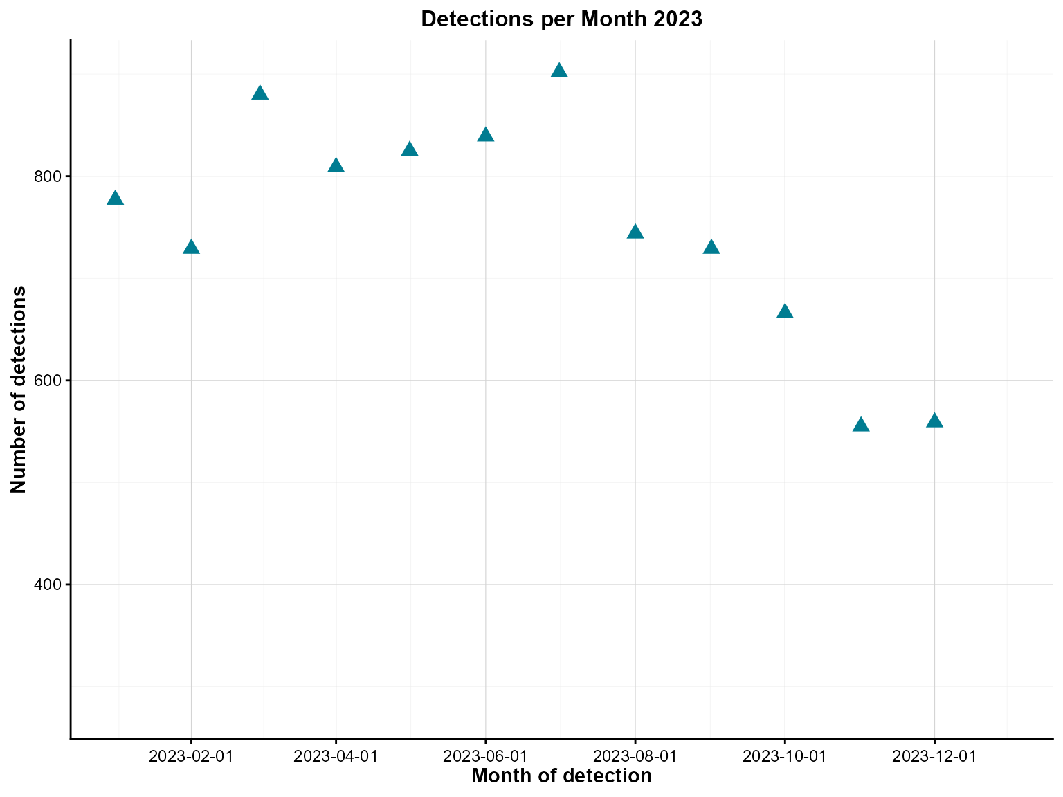
Monthly detections with point markers across 2023.

Interpretation: This point chart shows the relationship between time and monthly detections, revealing temporal patterns and any outliers in the data.

Example 2: Interactive point chart

Interactive point charts allow users to explore data dynamically, with hover information and zooming capabilities.

Create the interactive point chart

point_chart(
  dynamic = TRUE,   # Create interactive plotly chart
  params = list(
    df = monthly_data,
    x = "specimen_month",
    y = "detections",
    point_colours = "#007C91",
    point_size = 3,
    x_limit_min = "2022-01-01",
    x_limit_max = "2023-12-31",
    chart_title = "Detections per Month 2022-2023",
    x_axis_title = "Month of detection",
    y_axis_title = "Number of detections",
    x_axis_date_breaks = "2 months"
  )
)

Interactive monthly detections with hover detail.

Interpretation: The interactive version allows detailed exploration of the temporal patterns, with hover information showing exact values for each month.

Example 3: Grouped point chart with confidence ribbons

Grouped point charts with confidence ribbons are excellent for comparing multiple categories while showing uncertainty estimates.

Prepare grouped data with confidence intervals

# Create grouped data with confidence intervals (as used in tests)
set.seed(123)
grouped_data <- epiviz::lab_data %>%
  group_by(specimen_month = lubridate::floor_date(specimen_date, 'month'),
           organism_species_name) %>%
  summarise(detections = n()) %>%
  ungroup() %>%
  mutate(
    offset = sample(10:50, n(), replace = TRUE),
    lower_limit = pmax(detections - offset, 0),
    upper_limit = detections + offset
  ) %>%
  select(-offset)

Create the grouped point chart with confidence ribbons

point_chart(
  dynamic = FALSE,  # Create static ggplot chart
  params = list(
    df = grouped_data,
    x = "specimen_month",
    y = "detections",
    group_var = "organism_species_name",  # Group by organism type
    point_colours = c("#007C91", "#8A1B61", "#FF7F32"),  # Colors for each group
    point_size = 3,
    x_limit_min = "2022-01-01",
    x_limit_max = "2023-12-31",
    chart_title = "Detections per Month 2022-2023",
    x_axis_title = "Month of detection",
    y_axis_title = "Number of detections",
    x_axis_date_breaks = "2 months",
    y_axis_break_labels = seq(0, 600, 100),  # Custom y-axis breaks
    x_axis_label_angle = 45,                 # Rotate x-axis labels
    # Confidence interval parameters
    ci = "ribbon",                           # Use ribbon for confidence intervals
    ci_lower = "lower_limit",                # Lower confidence limit column
    ci_upper = "upper_limit",                # Upper confidence limit column
    ci_colours = c("#007C91", "#8A1B61", "#FF7F32")  # Colors for confidence ribbons
  )
)

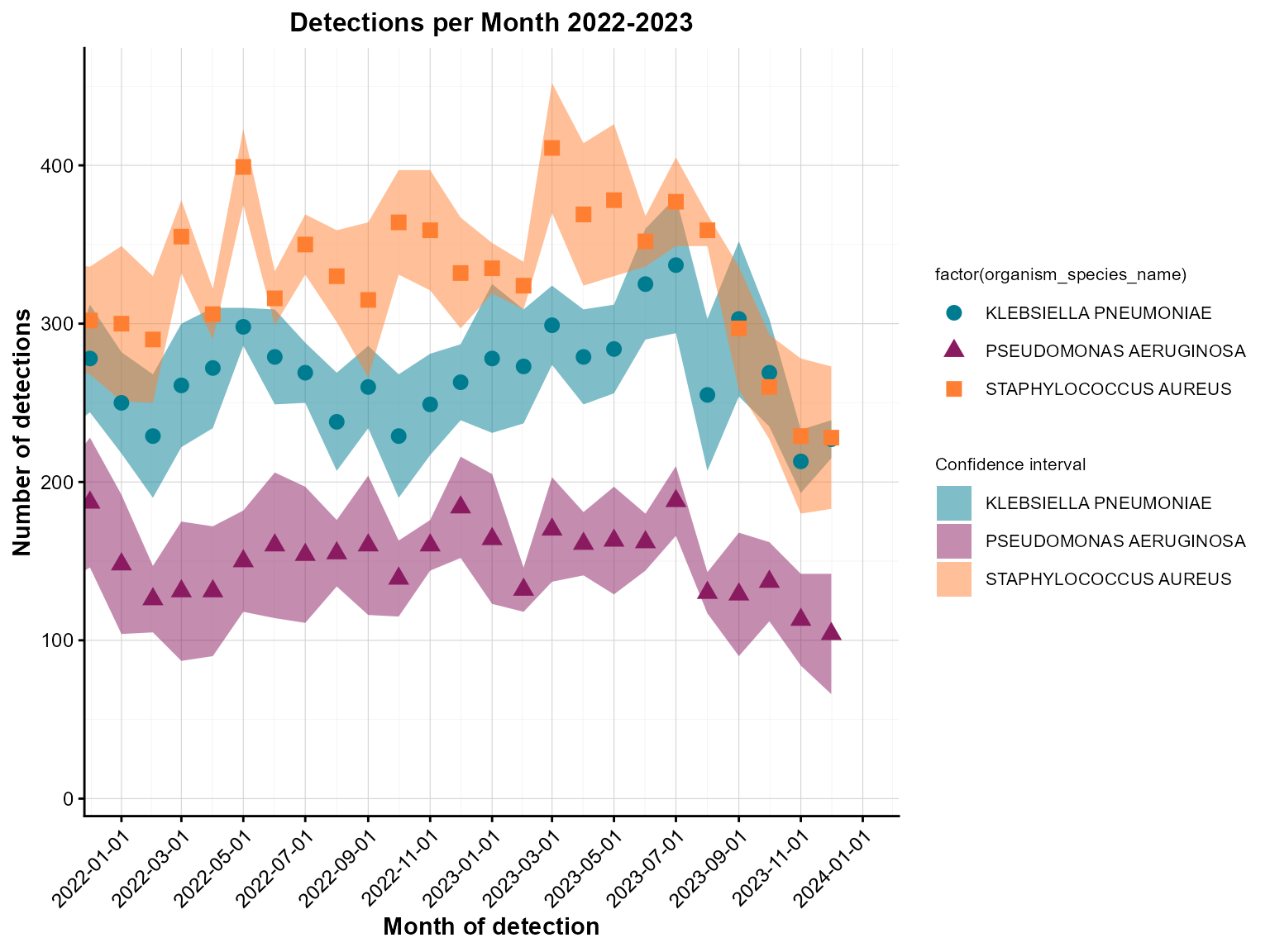
Grouped monthly detections with confidence ribbons.

Interpretation: This grouped point chart shows detections by organism type over time, with confidence ribbons indicating uncertainty around the estimates.

Example 4: Point chart with threshold lines

Threshold lines help identify data points that exceed or fall below important cutoffs, such as outbreak levels or target values.

Create the point chart with threshold lines

point_chart(
  dynamic = FALSE,  # Create static ggplot chart
  params = list(
    df = grouped_data,
    x = "specimen_month",
    y = "detections",
    group_var = "organism_species_name",
    point_colours = c("#007C91", "#8A1B61", "#FF7F32"),
    point_size = 3,
    x_limit_min = "2022-01-01",
    x_limit_max = "2023-12-31",
    chart_title = "Detections per Month 2022-2023",
    x_axis_title = "Month of detection",
    y_axis_title = "Number of detections",
    x_axis_date_breaks = "2 months",
    y_axis_break_labels = seq(0, 600, 100),
    x_axis_label_angle = 45,
    ci = "ribbon",
    ci_lower = "lower_limit",
    ci_upper = "upper_limit",
    ci_colours = c("#007C91", "#8A1B61", "#FF7F32"),
    # Threshold lines
    hline = c(450, 550),                    # Multiple threshold lines
    hline_colour = c("blue", "red"),        # Colors for each line
    hline_label = c("threshold 1", "threshold 2"),  # Labels for lines
    hline_label_colour = c("blue", "red")   # Label colors
  )
)

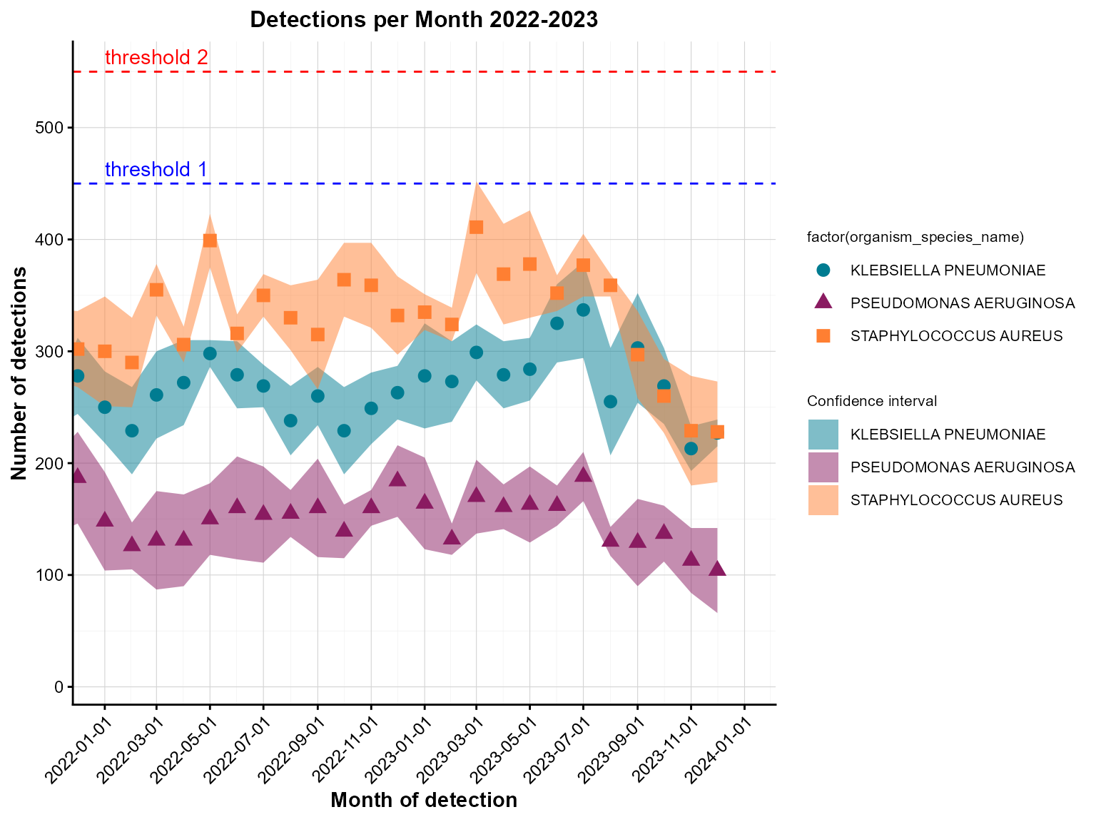
Grouped monthly detections with threshold lines.

Interpretation: This point chart includes threshold lines to identify months where detections exceeded specific levels, helping prioritize periods for further investigation.

Example 5: Interactive grouped point chart with all features

Interactive point charts with all features provide the most comprehensive view for surveillance dashboards and exploratory analysis.

Create the comprehensive interactive point chart

point_chart(
  dynamic = TRUE,   # Create interactive plotly chart
  params = list(
    df = grouped_data,
    x = "specimen_month",
    y = "detections",
    group_var = "organism_species_name",
    point_colours = c("#007C91", "#8A1B61", "#FF7F32"),
    point_size = 3,
    x_limit_min = "2022-01-01",
    x_limit_max = "2023-12-31",
    chart_title = "Detections per Month 2022-2023",
    x_axis_title = "Month of detection",
    y_axis_title = "Number of detections",
    x_axis_date_breaks = "2 months",
    y_axis_break_labels = seq(0, 600, 100),
    x_axis_label_angle = 45,
    ci = "ribbon",
    ci_lower = "lower_limit",
    ci_upper = "upper_limit",
    ci_colours = c("#007C91", "#8A1B61", "#FF7F32"),
    hline = c(450, 550),
    hline_colour = c("blue", "red"),
    hline_label = c("threshold 1", "threshold 2"),
    hline_label_colour = c("blue", "red")
  )
)

Interactive grouped point chart with confidence ribbons and thresholds.

Interpretation: This comprehensive interactive point chart combines grouped data visualization with confidence ribbons and threshold lines, providing multiple layers of information for surveillance analysis.

Tips for point charts

1. Data preparation: Always aggregate your data appropriately before passing it to point_chart(). The function expects pre-calculated counts or values.

2. Date handling: Use lubridate::floor_date() to create consistent time periods for aggregation, as shown in the test examples.

3. Confidence intervals: Use ci = "ribbon" with ci_lower and ci_upper parameters to add confidence ribbons around your data points.

4. Threshold lines: Use hline parameters to add horizontal reference lines for alert levels or targets:

   hline = c(450, 550),
   hline_colour = c("blue", "red"),
   hline_label = c("threshold 1", "threshold 2")

5. Grouping: Use group_var to create multiple series for comparison. Each group will get a different color.

6. Point styling: Customize appearance with:

   • point_colours: Colors for points (vector for multiple groups)
   • point_size: Size of points
   • ci_colours: Colors for confidence ribbons

7. Axis limits: Use x_limit_min and x_limit_max to control the x-axis range for better focus on relevant time periods.

8. Interactive features: Set dynamic = TRUE for interactive charts with zooming, hovering, and filtering capabilities.

9. Axis formatting: Use x_axis_date_breaks and y_axis_break_labels to control how dates and values are displayed on the axes.

10. Label rotation: Use x_axis_label_angle to rotate date labels for better readability.

11. Confidence ribbon colors: Ensure ci_colours matches your point_colours for consistent visual representation.

12. Random confidence intervals: In the test examples, confidence intervals are generated randomly. In real applications, use appropriate statistical methods to calculate meaningful confidence intervals.