Legrand Ebola SEIHFR

Legrand_Ebola_SEIHFR()

A commonly used model in the literature to capture the dynamics of Ebola outbreaks is the SEIHFR model proposed by Legrand et al ⁷. There are two extra compartments on top of the SEIR: \(H\) for hospitializations and \(F\) for funerals. A total of ten parameters (with some describing the inverse) are required for the model.

Symbol	Process
\(\beta_{I}\)	Transmission rate in community
\(\beta_{H}\)	Transmission rate in hospital
\(\beta_{F}\)	Transmission rate in funeral
\(\gamma_{I}\)	(inverse) Onset to end of infectious
\(\gamma_{D}\)	(inverse) Onset to death
\(\gamma_{H}\)	(inverse) Onset of hospitilization
\(\gamma_{F}\)	(inverse) Death to burial
\(\alpha\)	(inverse) Duration of the incubation period
\(\theta\)	Proportional of cases hospitalized
\(\delta\)	Case–ftality ratio

The (inverse) denotes the parameter should be inverted to make epidemiological sense. We use the parameters in their more natural from in Legrand_Ebola_SEIHFR() and replace all the \(\gamma\)’s with \(\omega\)’s, i.e. \(\omega_{i} = \gamma_{i}^{-1}\) for \(i \in \{I,D,H,F\}\). We also used \(\alpha^{-1}\) in our model instead of \(\alpha\) so that reading the parameters directly gives a more intuitive meaning. There are five additional parameters that is derived. The two derived case fatality ratio as

\[\begin{split}\begin{aligned} \delta_{1} &= \frac{\delta \gamma_{I}}{\delta \gamma_{I} + (1-\delta)\gamma_{D}} \\ \delta_{2} &= \frac{\delta \gamma_{IH}}{\delta \gamma_{IH} + (1-\delta)\gamma_{DH}}, \end{aligned}\end{split}\]

with an adjusted hospitalization parameter

\[\theta_{1} = \frac{\theta(\gamma_{I}(1-\delta_{1}) + \gamma_{D}\delta_{1})}{\theta(\gamma_{I}(1-\delta_{1}) + \gamma_{D}\delta_{1}) + (1-\theta)\gamma_{H}},\]

and the derived infectious period

\[\begin{split}\begin{aligned} \gamma_{IH} &= (\gamma_{I}^{-1} - \gamma_{H}^{-1})^{-1} \\ \gamma_{DH} &= (\gamma_{D}^{-1} - \gamma_{H}^{-1})^{-1}. \end{aligned}\end{split}\]

Now we are ready to state the full set of ODEs,

\[\begin{split}\begin{aligned} \frac{dS}{dt} &= -N^{-1} (\beta_{I}SI + \beta_{H}SH + \beta_{F}(t) SF) \\ \frac{dE}{dt} &= N^{-1} (\beta_{I}SI + \beta_{H}SH + \beta_{F}(t) SF) - \alpha E \\ \frac{dI}{dt} &= \alpha E - (\gamma_{H} \theta_{1} + \gamma_{I}(1-\theta_{1})(1-\delta_{1}) + \gamma_{D}(1-\theta_{1})\delta_{1})I \\ \frac{dH}{dt} &= \gamma_{H}\theta_{1}I - (\gamma_{DH}\delta_{2} + \gamma_{IH}(1-\delta_{2}))H \\ \frac{dF}{dt} &= \gamma_{D}(1-\theta_{1})\delta_{1}I + \gamma_{DH}\delta_{2}H - \gamma_{F}F \\ \frac{dR}{dt} &= \gamma_{I}(1-\theta_{1})(1-\delta_{1})I + \gamma_{IH}(1-\delta_{2})H + \gamma_{F}F. \end{aligned}\end{split}\]

with \(\beta_{F}(t) = \beta_{F}\) if \(t > c\) and \(0\) otherwise. We use a slightly modified version by replacing the delta function with a sigmoid function namely, the logistic function

\[\beta_{F}(t) = \beta_{F} \left(1 - \frac{1}{1 + \exp(-\kappa (t - c))} \right)\]

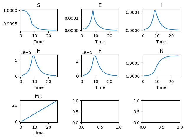
A brief example is given here:

import numpy

from pygom import common_models

x0 = [1.0, 3.0/200000.0, 0.0, 0.0, 0.0, 0.0, 0.0]

t = numpy.linspace(1, 25, 100)

ode = common_models.Legrand_Ebola_SEIHFR([('beta_I',0.588),
                                          ('beta_H',0.794),
                                          ('beta_F',7.653),
                                          ('omega_I',10.0/7.0),
                                          ('omega_D',9.6/7.0),
                                          ('omega_H',5.0/7.0),
                                          ('omega_F',2.0/7.0),
                                          ('alphaInv',7.0/7.0),
                                          ('delta',0.81),
                                          ('theta',0.80),
                                          ('kappa',300.0),
                                          ('interventionTime',7.0)])

ode.initial_values = (x0, t[0])

solution = ode.integrate(t)

ode.plot()

Note

We have standardized the states so that the number of susceptible is 1 and equal to the whole population, i.e. \(N\) does not exist in our set of ODEs.