SEIR, birth, death, periodic, waning and introductions#
SEIR_Birth_Death_Periodic_Waning_Intro()
This model includes relatively more detail than the other pre-defined models provided and may serve as a template for more complex models.
In addition to the processes of births, deaths and seasonal driving, we have included (i) immune waning, which transitions recovered individuals back to susceptible at a rate \(w\) and (ii) an external force of infection, which allows individuals to be infected from outside the population (analogous to case importation) at a rate \(\epsilon\).
We solve this set of equations stochastically:
from pygom import common_models
import matplotlib.pyplot as plt
import numpy as np
import math

# Set up PyGOM object

# Parameters

## population
n_pop=1e6

## Seasonal driving
beta0=0.3               # R0 avg = beta0/gamma =1.2, R0 min = (beta0-delta)/gamma=0.8, R0 max = (beta0+delta)/gamma=1.6
delta=0.1
period=365

## Virus
alpha=1/2
gamma=1/4
mu=0.01/365
w=1/(2*365)              # waning rate, immunity lasts ~ 2 years.
epsilon=50/(365*n_pop)   # attack rate:approximately 100*n_sus*365/(365*n_pop)=100*frac_sus
                         # infections from external sources per year (approx 1 per week, just enough
                         # to spark an epidemic when winter arrives)

model = common_models.SEIR_Birth_Death_Periodic_Waning_Intro({'beta0':beta0,
                                                              'delta':delta,
                                                              'period':period,
                                                              'alpha':alpha,
                                                              'gamma':gamma,
                                                              'mu':mu,
                                                              'w':w,
                                                              'ar': epsilon})

# Time range and increments
tmax=365*20                           # maximum time over which to run solver
dt=10                                 # output timestep
n_timestep=math.ceil(tmax/dt)         # number of iterations
t = np.linspace(0, tmax, n_timestep)  # times at which solution will be evaluated

# Initial conditions
x0 = [n_pop, 0, 0, 0, n_pop]

model.initial_values = (x0, t[0])

np.random.seed(1)

n_sim=2
solution, jump, simT = model.solve_stochast(t, n_sim, full_output=True)
Show code cell output
Illegal jump, x: [1.000024e+06 2.000000e+00 0.000000e+00 0.000000e+00 1.000026e+06], new x: [ 1.000032e+06 -2.000000e+00  4.000000e+00  0.000000e+00  1.000034e+06]
Illegal jump, x: [1.000069e+06 0.000000e+00 3.000000e+00 5.000000e+00 1.000077e+06], new x: [ 1.000063e+06  5.000000e+00 -1.000000e+00  9.000000e+00  1.000076e+06]
Illegal jump, x: [1.000047e+06 4.000000e+00 3.000000e+00 1.000000e+01 1.000064e+06], new x: [ 1.000072e+06 -1.000000e+00  5.000000e+00  1.400000e+01  1.000090e+06]
Illegal jump, x: [9.999840e+05 6.000000e+00 6.000000e+00 5.300000e+01 1.000049e+06], new x: [ 9.999700e+05 -1.000000e+00  1.600000e+01  5.400000e+01  1.000039e+06]
Illegal jump, x: [7.458530e+05 2.000000e+01 3.100000e+01 2.546380e+05 1.000542e+06], new x: [ 7.491890e+05 -2.200000e+01  4.200000e+01  2.513270e+05  1.000536e+06]
Illegal jump, x: [7.551960e+05 2.200000e+01 5.300000e+01 2.452370e+05 1.000508e+06], new x: [ 7.593740e+05  3.500000e+01 -4.000000e+00  2.410880e+05  1.000493e+06]
Illegal jump, x: [7.551970e+05 2.200000e+01 5.300000e+01 2.452360e+05 1.000508e+06], new x: [ 7.592690e+05  8.300000e+01 -3.000000e+00  2.411400e+05  1.000489e+06]
Illegal jump, x: [7.640260e+05 1.400000e+01 4.400000e+01 2.364370e+05 1.000521e+06], new x: [ 7.65920e+05  5.80000e+01 -4.00000e+00  2.34556e+05  1.00053e+06]
Illegal jump, x: [7.67639e+05 2.80000e+01 4.20000e+01 2.32831e+05 1.00054e+06], new x: [ 7.701370e+05 -3.000000e+00  6.500000e+01  2.303990e+05  1.000598e+06]
Illegal jump, x: [7.81219e+05 3.10000e+01 5.20000e+01 2.19198e+05 1.00050e+06], new x: [ 7.842350e+05 -9.000000e+00  8.100000e+01  2.162050e+05  1.000512e+06]
Illegal jump, x: [8.068120e+05 2.400000e+01 5.000000e+01 1.937060e+05 1.000592e+06], new x: [ 8.118410e+05 -1.200000e+01  2.600000e+01  1.887500e+05  1.000605e+06]
Illegal jump, x: [8.172220e+05 1.300000e+01 2.300000e+01 1.832690e+05 1.000527e+06], new x: [ 8.208820e+05 -1.400000e+01  4.600000e+01  1.796150e+05  1.000529e+06]
Illegal jump, x: [8.281030e+05 6.000000e+00 1.700000e+01 1.724920e+05 1.000618e+06], new x: [ 8.323950e+05  3.200000e+01 -2.200000e+01  1.682580e+05  1.000663e+06]
Illegal jump, x: [8.47987e+05 2.70000e+01 2.50000e+01 1.52601e+05 1.00064e+06], new x: [ 8.484980e+05 -4.000000e+00  5.400000e+01  1.520860e+05  1.000634e+06]
Illegal jump, x: [8.876300e+05 5.300000e+01 1.050000e+02 1.129780e+05 1.000766e+06], new x: [ 8.884230e+05 -1.000000e+00  1.270000e+02  1.122270e+05  1.000776e+06]
Illegal jump, x: [8.090790e+05 3.100000e+01 5.000000e+01 1.915120e+05 1.000672e+06], new x: [ 8.110180e+05 -5.000000e+00  8.300000e+01  1.895800e+05  1.000676e+06]
Illegal jump, x: [8.090790e+05 3.000000e+01 5.100000e+01 1.915120e+05 1.000672e+06], new x: [ 8.11620e+05 -1.10000e+01  1.10000e+02  1.88891e+05  1.00061e+06]
Illegal jump, x: [8.583830e+05 3.800000e+01 6.200000e+01 1.415800e+05 1.000063e+06], new x: [ 8.596920e+05 -7.000000e+00  9.800000e+01  1.402600e+05  1.000043e+06]
Illegal jump, x: [1.000003e+06 2.000000e+00 0.000000e+00 0.000000e+00 1.000005e+06], new x: [ 1.000003e+06 -4.000000e+00  6.000000e+00  0.000000e+00  1.000005e+06]
Illegal jump, x: [1.000002e+06 2.000000e+00 0.000000e+00 0.000000e+00 1.000004e+06], new x: [ 1.000019e+06 -6.000000e+00  8.000000e+00  0.000000e+00  1.000021e+06]
Illegal jump, x: [1.000003e+06 2.000000e+00 0.000000e+00 0.000000e+00 1.000005e+06], new x: [ 1.000009e+06 -1.000000e+00  4.000000e+00  0.000000e+00  1.000012e+06]
Illegal jump, x: [9.99994e+05 0.00000e+00 2.00000e+00 0.00000e+00 9.99996e+05], new x: [ 1.000008e+06  3.000000e+00 -3.000000e+00  5.000000e+00  1.000013e+06]
Illegal jump, x: [9.99975e+05 2.00000e+00 3.00000e+00 2.00000e+00 9.99982e+05], new x: [ 9.99954e+05 -4.00000e+00  8.00000e+00  5.00000e+00  9.99963e+05]
Illegal jump, x: [9.99974e+05 2.00000e+00 3.00000e+00 2.00000e+00 9.99981e+05], new x: [ 9.99940e+05  7.00000e+00 -2.00000e+00  8.00000e+00  9.99953e+05]
Illegal jump, x: [8.43410e+05 4.80000e+01 7.80000e+01 1.56447e+05 9.99983e+05], new x: [ 8.44359e+05 -1.00000e+00  1.26000e+02  1.55526e+05  1.00001e+06]
Illegal jump, x: [8.52753e+05 7.30000e+01 1.22000e+02 1.46966e+05 9.99914e+05], new x: [ 8.53870e+05 -4.00000e+00  2.05000e+02  1.45836e+05  9.99907e+05]
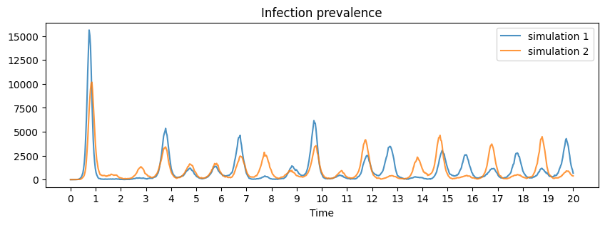
Plotting the infection prevalence over 2 simulations reveals that an initially large epidemic is eventually succeeded by a series of fairly regular annual epidemics of varying sizes.
Show code cell source
f, ax = plt.subplots(figsize=(10, 3))

ax.set_xlabel("Time")
ax.set_title("Infection prevalence")
ax.plot(t/365, solution[0][:,2], alpha=0.8, label="simulation 1")
ax.plot(t/365, solution[1][:,2], alpha=0.8, label="simulation 2")
plt.xticks(np.arange(0, 21, 1.0))
ax.legend()
plt.show()