SIS, periodic#
This is an extension of the SIS model which incorporates a periodic infection rate, \(\beta(t)\). This could be used to mimic seasonal variation in infectivity due to yearly contact rate patterns or climate drivers, for example. We define \(\beta(t)\) as follows:
\[\begin{aligned}
\beta(t) &= \beta_0 \left(1+\delta \cos \left(\frac{2 \pi t}{P} \right) \right)
\end{aligned}\]
where \(\beta_0\) is the baseline infection rate, \(\delta\) is the magnitude of oscillations from the baseline (\(-1<\delta<1\) so that \(\beta>0\)) and \(P\) is the period of oscillations.
Also, note how we can use \(I+S=N\) to eliminate the equation for \(S\):
\[\begin{split}\begin{aligned}
\frac{\mathrm{d}I}{\mathrm{d}t} &= (\beta(t)N - \alpha) I - \beta(t)I^{2} \\
\end{aligned}\end{split}\]
In Heathcote’s classical model, \(\gamma=1\) and:
\[\begin{split}\begin{aligned}
\beta(t) &= 2 - 1.8 \cos(5t) \\
&= 2\left(1 - 0.9 \cos \left( \frac{2 \pi t}{ \frac{2 \pi}{5} } \right) \right)
\end{aligned}\end{split}\]
so that \(\beta_0=2\), \(\delta=0.9\) and \(P=\frac{2 \pi}{5}\).
from pygom import common_models
import matplotlib.pyplot as plt
import numpy as np
import math

# Set up PyGOM object
n_pop=1e4

ode = common_models.SIS_Periodic({'gamma':1, 'beta0':2, 'delta':0.9, 'period':(2*math.pi/5), 'N':n_pop})

# Time range and increments
tmax=10                               # maximum time over which to run solver
dt=0.01                               # timestep
n_timestep=math.ceil(tmax/dt)         # number of iterations
t = np.linspace(0, tmax, n_timestep)  # times at which solution will be evaluated

# Initial conditions
i0=0.1*n_pop
s0=n_pop-i0
x0 = [s0, i0]

ode.initial_values = (x0, t[0])
solution=ode.solve_determ(t[1::])
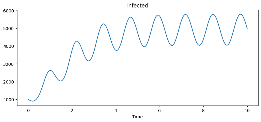
We plot the infected trajectory which shows periodic evolution.
Show code cell source
f, ax = plt.subplots(figsize=(10, 4))

ax.set_xlabel("Time")
ax.set_title("Infected")
ax.plot(t, solution[:,1])
plt.show()