Lotka Volterra

The model Lotka_Volterra() is a basic predator and prey model ⁹. This is more commonly expressed in terms of predator and prey population area densities, \(x\) and \(y\) respectively, though we define the model in terms of absolute numbers, \(X\) and \(Y\), in a given area, \(A\). This decision to define in terms of population numbers, rather than densities, permits us to perform stochastic simulations.

\[\begin{split}\begin{aligned} \frac{\mathrm{d} X}{\mathrm{d} t} &= \alpha X - \frac{\beta X Y}{A} \\ \frac{\mathrm{d} Y}{\mathrm{d} t} &= -\gamma Y + \frac{\delta X Y}{A} \end{aligned}\end{split}\]

We first solve this model for the deterministic case:

from pygom import common_models
import numpy as np
import matplotlib.pyplot as plt
import math

# Initial populations
x0=[40, 20]

# Parameters from a snowshoe hare / Canadian lynx system
# https://mc-stan.org/users/documentation/case-studies/lotka-volterra-predator-prey.html
alpha=0.545
beta=0.028
gamma=0.803
delta=0.024

# scale up the population (this will need scaling in the predation parameters)
scale=10

x0 = [x * scale for x in x0]
beta=beta/scale
delta=delta/scale


ode = common_models.Lotka_Volterra({'alpha':alpha,
                                    'beta':beta,
                                    'gamma':gamma,
                                    'delta':delta})

tmax=50                               # maximum time over which to run solver
dt=0.1                                # timestep
n_timestep=math.ceil(tmax/dt)         # number of iterations
t = np.linspace(0, tmax, n_timestep)  # times at which solution will be evaluated

ode.initial_values = (x0, t[0])

solution = ode.solve_determ(t[1::])

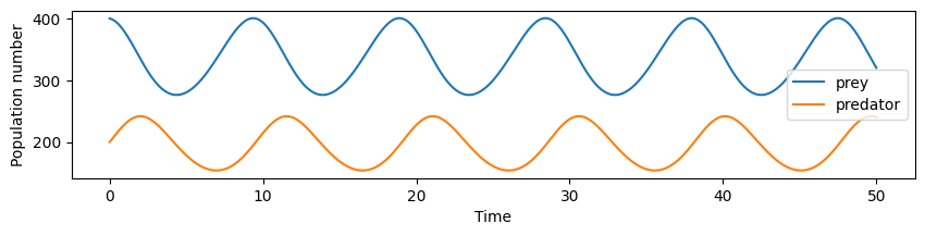
We see that the predator and prey populations show periodic behaviour with a phase shift between them.

Show code cell source Hide code cell source

f, ax = plt.subplots(figsize=(10, 2))

ax.set_xlabel("Time")
ax.set_ylabel("Population number")
ax.plot(t, solution[:,0], label="prey")
ax.plot(t, solution[:,1], label="predator")
ax.legend()
plt.show()

We can also see how the system evolves stochastically

np.random.seed(1)

n_sim=1
solution, jump, simT = ode.solve_stochast(t, n_sim, full_output=True)

f, ax = plt.subplots(figsize=(10, 2))

y=np.dstack(solution)

ax.set_xlabel("Time")
ax.set_ylabel("Population number")
ax.plot(t, y[:,0], label="prey")
ax.plot(t, y[:,1], label="predator")
ax.legend()
plt.show()

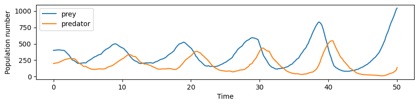
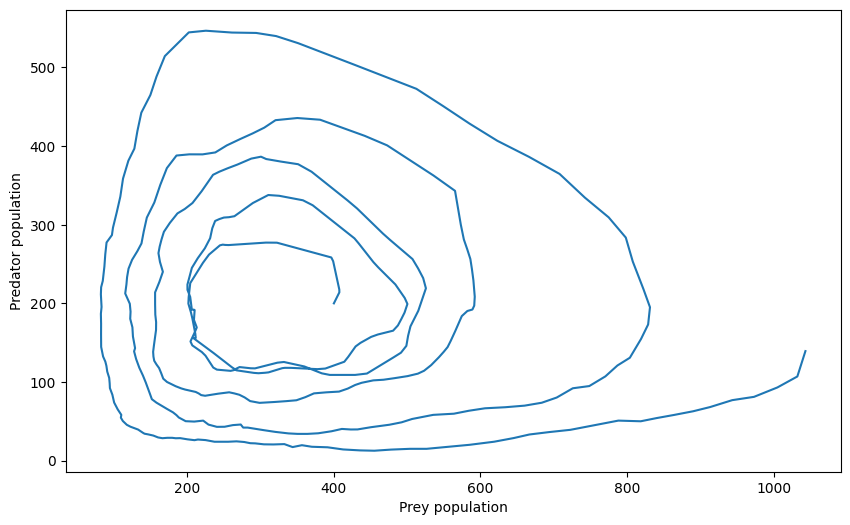
This appears to be unstable, since the populations undergo increasingly extreme peaks and troughs. This can be confirmed by examining a phase diagram, whereby the trajectory in state space spirals outwards.

f, ax = plt.subplots(figsize=(10, 6))
ax.plot(y[:,0], y[:,1])
ax.set_xlabel("Prey population")
ax.set_ylabel("Predator population")
plt.show()